A few months ago I release this funky song Happiness is just one boom away which is an experimental track from my album The AI Band. I dive into the irony of economic growth and its hidden costs. This song explores justice, inequality, and the environmental impact of so-called progress.
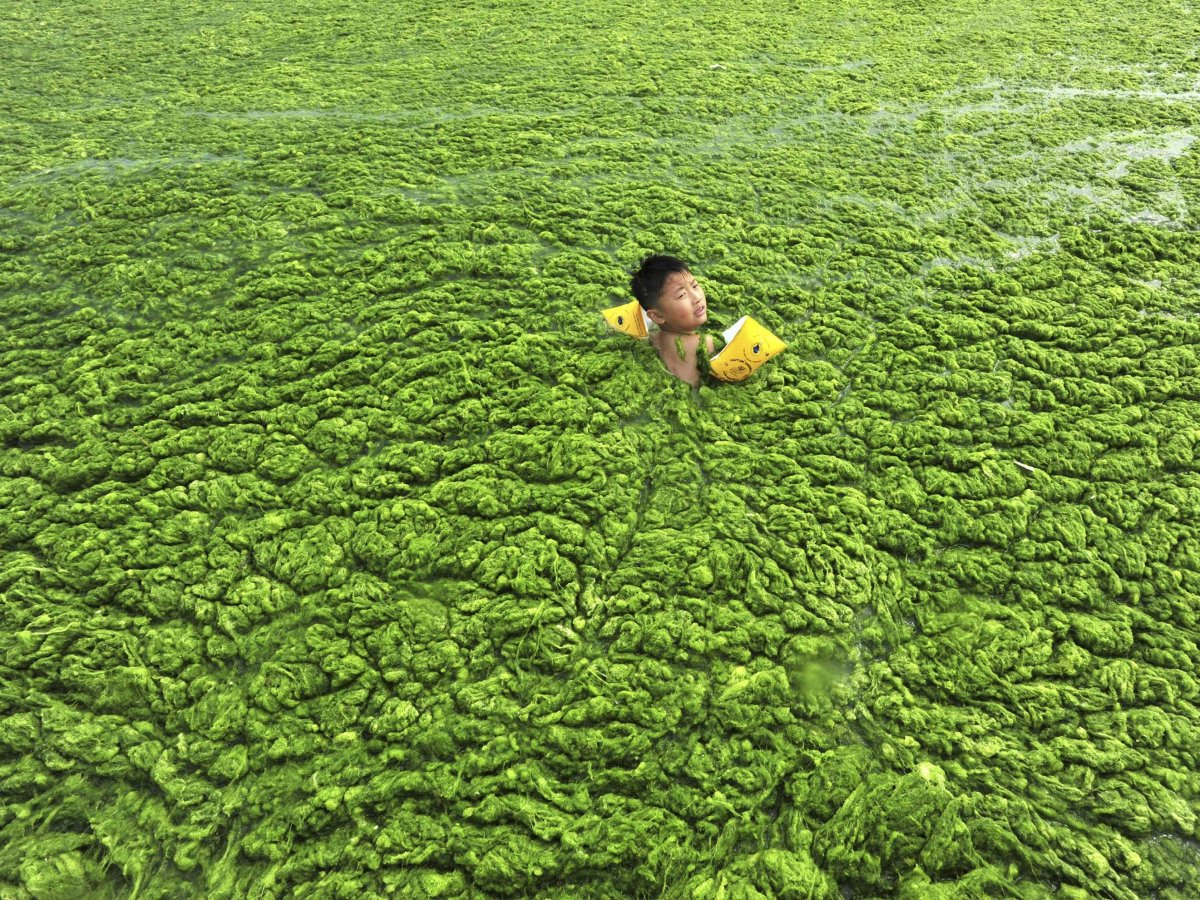
After that I was wondering. Not too long ago, music promotion was all about physical copies, radio play, and word of mouth. Artists handed out mixtapes, played countless live gigs, and relied on record labels to push their music onto radio stations and into stores. Magazines, TV appearances, and even flyers played a crucial role in getting a song heard. Discovery was organic—people found music through recommendations from friends, record store owners, or simply by stumbling upon a great band at a live show.
Fast forward to today, and the game has completely changed. Algorithms now dictate what people listen to. Streaming platforms like Spotify, YouTube, and TikTok use data-driven recommendations, showing users songs based on what keeps them engaged the longest. Instead of DJs and critics deciding what gets exposure, it’s now AI-driven playlists, social media trends, and engagement metrics.
While this has opened doors for independent artists, allowing anyone to reach a global audience, it has also created a system where virality often matters more than musical depth. Artists are pushed to create content constantly, play to the algorithm, and tailor their sound to fit trends rather than artistic vision. Music discovery is faster than ever, but are we truly choosing what we listen to, or is the algorithm choosing for us?
It seems I can’t get out of the rabbit hole. Every time I release some video I get only a few views. I wonder, is my music really good? Bad? Is it my Youtube channel? Maybe, but what it is really ironic is the fact that I am in a video with more than 1 million views and people commented a lot about my playing.
Regardless, not giving up is the secret and I will be releasing my songs even without a good amount of views. Any positive comment is always a win and I am thankful for the few people that watched and liked.