Almost 10 years ago I was working with evolutionary strategies for tuning neural network for time series prediction when I became curious about error measures and the effects on the final forecast. In general, evolutionary algorithms use a fitness function that is based on a error measure. The objective is to get better individual(s) minimizing (or maximizing) the fitness function. Thus, to determine which model is “the best”, the performance of a trained model is evaluated against one or more criteria (e.g. error measure). However, the relation between the lowest error and “best model” is complex and should be applied according with the desirable goal (i.e. forecasting average, forecasting extremes, deviance measures, relative errors, etc.).
There is a journal paper which gives the description of the errors used in the ‘qualV’ package. This package has several implementations of quantitative validation methods. The paper (which is very interesting by the way), also has some examples of how the final results of the errors measures change when dealing with noise, shifts, nonlinear scaling, etc.
The objective of this post is just to show the problem, and raise the awareness when measuring the best model based on error only. Sometimes the minimization of one error measure does not guarantee the minimization of all other error measures and it even could lead to a pareto front. Here i am using some of the functions described in the paper and for simplicity i am comparing here only 4 errors measures: mean absolute error (MAE), root-mean-square error (RMSE), correlation coefficient (r) and mean absolute percentage error (MAPE). Each error measure is measuring a distinct characteristic of the time series and each of them has strong and weak points. I am using R version 3.3.2 (2016-10-31) on Ubuntu 16.04.
Case (i): Adding noise
Lets say we have the function with the original signal given by:
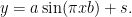
Using x=[0,1], a=1.5, b=2, and s=0.75 then:
x = seq(0,1,by=.005)
ysignal = 1.5*sin(pi*2*x)+0.75
plot(x,ysignal,main = "Main signal")
We should change the original signal and check how this will affect the final result. If the “forecast” is the same as the signal then all the errors should be 0. Thus applying some noise to the signal s=(0.75+noise), where noise comes from a Gaussian function with mean=0 and standard deviation =0.2, and comparing with the original signal we get:
library(qualV)
n = 0.2 #noise level
noise = rnorm(length(x),sd=n)
ynoise = ysignal+noise
par(mfrow=c(1,2))
range.yy <- range(c(ysignal,ynoise))
plot(x,ysignal,type='l',main = "Adding noise"); lines(x,ynoise,col=2)
plot(ynoise,ysignal,ylim=range.yy,xlim=range.yy,main = "Signal vs Forecast") 
round(MAE(ysignal,ynoise),2)
## [1] 0.16
round(RMSE(ysignal,ynoise),2)
## [1] 0.21
round(cor(ysignal,ynoise),2)
## [1] 0.98
round(MAPE(ysignal,ynoise),2)
## [1] 40.65
Case (ii): Shifting the signal
Lets apply a shift on the values of the original signal. With s=0.95 we have:
yshift = ysignal+0.2

round(MAE(ysignal,yshift),2)
## [1] 0.2
round(RMSE(ysignal,yshift),2)
## [1] 0.2
round(cor(ysignal,yshift),2)
## [1] 1
round(MAPE(ysignal,yshift),2)
## [1] 60.95
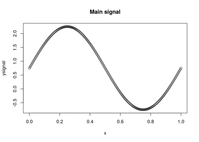
Case (iii): shift + rescale
Lets apply a shift and also rescale the values of the original signal. Doing a=0.8 and s=0.95 we have:
yresshift = 0.8*ysignal+0.2
round(MAE(ysignal,yresshift),2)
## [1] 0.19
round(RMSE(ysignal,yresshift),2)
## [1] 0.22
round(cor(ysignal,yresshift),2)
## [1] 1
round(MAPE(ysignal,yresshift),2)
## [1] 61.66
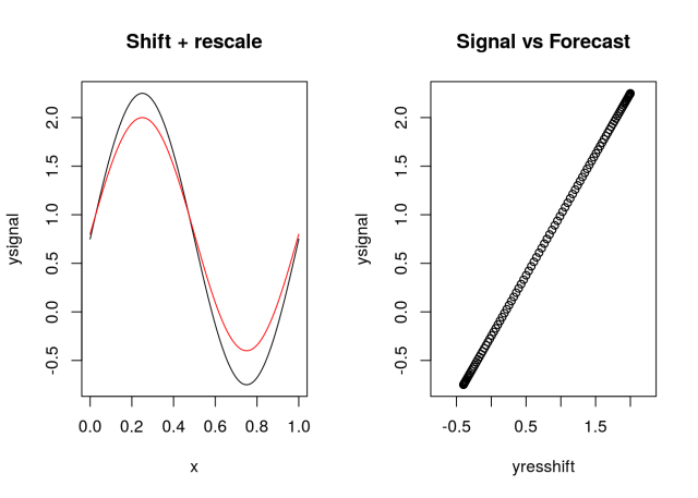
Case (iv): Changing the frequency
In this case lets vary slightly the frequency of the original signal making b=2.11:
yfreq = 1.5*sin(pi*2.11*x)+0.75
round(MAE(ysignal,yfreq),2)
## [1] 0.17
round(RMSE(ysignal,yfreq),2)
## [1] 0.22
round(cor(ysignal,yfreq),2)
## [1] 0.98
round(MAPE(ysignal,yfreq),2)
## [1] 89.33
Each case has the original series (in black) and the possible “forecast” (in red). I also plotted the original series (signal) versus the residual series. Which case would you pick as the best forecast? What is your assumption?
